Global profile mode

Sometimes all you want is a spatially-integrated spectrum of a source. The GlobalProfile class offers a simplified setup of MARTINI for this purpose.

Assumptions and limitations

In order to offer a simpler and faster way to produce a spectrum, the GlobalProfile class makes some assumptions:

No spatial aperture is assumed. Every particle in the source contributes to the spectrum (unless it falls outside of the spectral bandwidth).

The positions of particles are still used to calculate the line-of-sight vector and the velocity along this direction.

There is therefore no need or way to specify a beam or SPH kernel as with the main Martini class. It is also not possible to use MARTINI’s noise modules with this class. If these restrictions are found to be too limiting, the best course of action is to produce a spatially-resolved mock observation and derive the spectrum from those data as would be done with “real” observations. For example, if the spectrum within a spatial mask defined by a signal-to-noise or other cut is desired, or if spatially-dependent effects like primary beam attenuation are relevant, then the GlobalProfile class should not be used. The GlobalProfile class is mainly intended to efficiently provide a “quick look” at the spectrum, or a reference “ideal” spectrum.

Usage

The source and spectral model modules should be set up as for a full MARTINI mock observation. The beam, noise and sph_kernel modules are not relevant. The datacube module is not used, but a subset of its configuration options are instead given directly to the GlobalProfile. Schematically, an example initialisation looks like:

from martini import GlobalProfile
from martini.sources import SPHSource
from martini.spectral_models import GaussianSpectrum

source = SPHSource(...)
spectral_model = GaussianSpectrum(...)

gp = GlobalProfile(
    source=source,
    spectral_model=spectral_model,
    n_channels=64,
    channel_width=10 * U.km * U.s**-1,
    spectral_centre=source.vsys,
)

The arguments to the other modules are omitted here (replaced with ...), check the documentation pages of each module for details. Here the spectrum will be centred on the source systemic velocity, but an explicit frequency or Doppler velocity value could be given instead. The units of the channel_width argument determines whether the resulting spectrum will have channels evenly spaced in frequency (if channel_width has dimensions of frequency) or velocity (if it has dimensions of speed).

Inserting the source

The spectrum can be accessed through the spectrum attribute:

gp.spectrum

If it has not yet been calculated, it will be calculated when accessed. The calculation can be explicitly forced with:

gp.insert_source_in_spectrum()

but this is not usually necessary. In addition to the spectrum itself, the centres and edges of the channels are available as:

gp.channel_mids
gp.channel_edges

respectively. These arrays will have dimensions of frequency or velocity depending on the units of the channel_width argument passed to GlobalProfile on initialization. You can obtain the channel edges or centres in your preferred dimensions with:

gp.frequency_channel_mids
gp.frequency_channel_edges
gp.velocity_channel_mids
gp.velocity_channel_edges

Parallelization

The core loop in the source insertion function is a loop over pixels. Since parallelization is implemented for this loop, and for a GlobalProfile there is a single pixel, parallelization is not available in this mode.

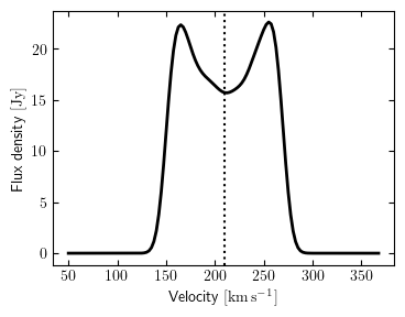
Quick plot of the spectrum

As a convenience, a function is provided to make a quick plot showing the spectrum. Whether the systemic velocity of the source (as reported by source.vsys) is shown by a vertical dotted line is controlled by the show_vsys argument. The channels argument (either "velocity" or "frequency") determines the units of the spectral axis in the figure.

from martini import demo_source, GlobalProfile
from martini.spectral_models import GaussianSpectrum

source = demo_source(N=20000)  # create a simple disc with 20000 particles
gp = GlobalProfile(
    source=source,
    spectral_model=GaussianSpectrum(sigma=7 * U.km * U.s**-1),
    n_channels=128,
    channel_width=2.5 * U.km * U.s**-1,
    spectral_centre=source.vsys,
    channels="velocity",
)
gp.plot_spectrum(
    show_vsys=True,
)

The resulting figure is returned by the function, or can be directly saved to file with the save argument (e.g. save="myplot.png" or save="myplot.pdf"). This example looks like: