Martini: core routines

The Martini class is the central element of MARTINI.

Putting it all together

Once all of the component modules are set up, creating an instance of Martini is straightforward, looking something like this:

source = SPHSource(...)
datacube = DataCube(...)
beam = GaussianBeam(...)
noise = GaussianNoise(...)
sph_kernel = GaussianKernel(...)
spectral_model = GaussianSpectrum(...)

m = Martini(
    source=source,
    datacube=datacube,
    beam=beam,
    noise=noise,
    sph_kernel=sph_kernel,
    spectral_model=spectral_model,
)

The arguments to the various modules are omitted here (replaced with ...), check the documentation pages of each module for details. The source, datacube, sph_kernel and spectral_model arguments are mandatory. The beam is optional in case you want an “intrinsic” observation of the source without convolution with a beam, and the noise is also optional in case you don’t want any in your mock observation (or perhaps want to later insert your mock into an observed noise cube). There is one more optional argument quiet (defaulting to False) that can be switched on for batch jobs where you don’t want any log messages.

A few things happen behind the scenes when the Martini object is initialized:

• First, if you provided a beam, your DataCube instance is padded in preparation for convolution with the beam. This is because a beam centred near the edge of the region of interest will pick up flux from outside of it, so MARTINI needs to fill a buffer region. This padding will be removed after convolution, or before any output files are written, but you may notice that your datacube doesn’t have the shape that you expect if you inspect it closely in the interim.

• Second, the source is moved to its orientation and location in the “sky” through a series of rotations and translations (in both position and velocity). The source modules allow for some inspection of the particles before making a mock observation (see source module documentation pages). This is almost always best done before passing the source to Martini.

• Next, the source is checked for particles that are guaranteed not to contribute to the datacube because they have no overlap with it in position (including their smoothing kernel and the padding region) and/or velocity (including spectral broadening). This speeds up later calculations, but you may notice that some particles have disappeared from your source object.

• Finally, the spectra of all (remaining) particles are calculated on the spectral axis grid. For sources with many particles this can take a bit of time, but the calculation is vectorized and so scales efficiently to large numbers of particles.

Mock observation preview

Similar to the preview functionality of the source module, the Martini object has a preview function, but with the added feature that it can obtain information from the DataCube member to draw the boundaries of the observation. The following example sets up a Martini instance similar to the one used in MARTINI’s demo() and generates a preview figure.

import numpy as np
import astropy.units as U
from martini import demo_source, DataCube, Martini
from martini.beams import GaussianBeam
from martini.noise import GaussianNoise
from martini.spectral_models import GaussianSpectrum
from martini.sph_kernels import CubicSplineKernel

source = demo_source(N=20000)  # create simple disc with 20000 particles
# a random rotation matrix:
rotmat = np.array(
    [
        [-0.20808178, -0.97804544, -0.01136216],
        [0.02991471, -0.01797457, 0.99939083],
        [0.97765387, -0.20761513, -0.03299812],
    ]
            )
# apply it so that the source has no particular orientation:
source.rotate(rotmat=rotmat)

datacube = DataCube(
    n_px_x=128,
    n_px_y=128,
    n_channels=32,
    px_size=10.0 * U.arcsec,
    channel_width=10.0 * U.km * U.s**-1,
    velocity_centre=source.vsys,
)

beam = GaussianBeam(
    bmaj=30.0 * U.arcsec, bmin=30.0 * U.arcsec, bpa=0.0 * U.deg, truncate=4.0
)

noise = GaussianNoise(rms=3.0e-5 * U.Jy * U.beam**-1)

spectral_model = GaussianSpectrum(sigma=7 * U.km * U.s**-1)

sph_kernel = CubicSplineKernel()

m = Martini(
    source=source,
    datacube=datacube,
    beam=beam,
    noise=noise,
    spectral_model=spectral_model,
    sph_kernel=sph_kernel,
)

m.preview(fig=1)  # uses matplotlib `plt.figure(1)`

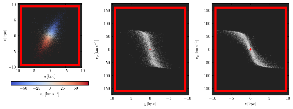
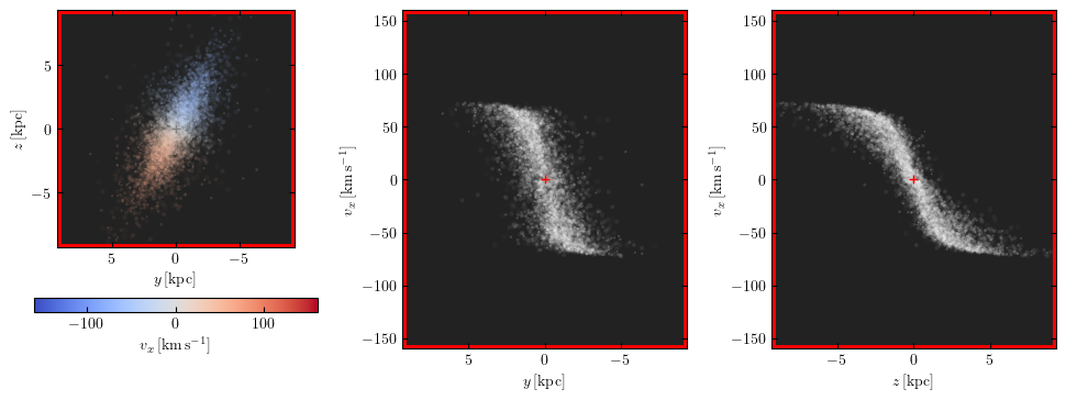
The red box marks the extent of the datacube in right ascension, declination and velocity. The axes limits can also be set to be equal to these extents by setting the keyword arguments lim="datacube" and vlim="datacube":

m.preview(fig=2, lim="datacube", vlim="datacube")

Check the source module documentation for further usage examples. Analogous usage works with the Martini preview() function (except that the extent of the data cube will be overlaid).

Inserting the source

This is the crucial step in creating a mock observation - the flux from the simulation particles needs to be added into the data cube. Since everything is already set up, all that needs to be done is to call martini.martini.Martini.insert_source_in_cube():

m.insert_source_in_cube()

Since this is the most computationally demanding step in MARTINI, a progress bar is displayed by default. This can be suppressed by passing the argument progressbar=False (or enabled with progressbar=True if Martini was initialized with quiet=True). There is another optional argument skip_validation. Setting this to True disables internal accuracy checks and is only intended for experimentation/prototyping and code development; it should never be used for science (and anyway doesn’t have any benefit in terms of e.g. speed).

Parallelization

Note

Available since v2.0.4.

The core loop in the source insertion function is embarassingly parallel. Parallel execution is implemented using the multiprocess package. You may need to install this, for instance pip install multiprocess to install from PyPI. To make use of the parallelization simply specify the number of processes to use, for example:

m.insert_source_in_cube(ncpu=2)

Executing with N processes is almost exactly N times faster than using a single process (provided that N cpus are available and otherwise idle). There is a small overhead to create processes (usually a second or less per process), usually dwarfed by the actual calculation by the time parallelization becomes a concern!

Progress bars work in principle in parallel mode, with one bar per process, although the formatting of the bars seems to occasionally get a bit glitchy.

Warning

multiprocess is not to be confused with multiprocessing - it is a fork of that package that, amongst other additional features, implements the object serialization used to pass data to/from processes with dill instead of pickle. This allows MARTINI’s object-oriented elements to be passed to processes. With multiprocessing, lots of internal bits would need to be moved to module-level global variables/functions, largely defeating the purpose of an object-oriented design.

Adding noise

If you passed a noise module instance to Martini, this is the time to use it, after inserting the source into the cube. Simply call add_noise():

m.add_noise()

This function has no required or optional parameters, so that’s all there is to it. Adding the noise should normally be done before convolving with the beam.

Convolving the beam

Since providing a beam is optional, so is actually performing the convolution operation. Assuming that this is a desired step, all that’s needed is to call convolve_beam():

m.convolve_beam()

This one is simple, with no parameters required or optional. You may notice that the datacube’s units change from something like \(\mathrm{Jy}\,\mathrm{arcsec}^2\) to \(\mathrm{Jy}\,\mathrm{beam}^{-1}\) during this step. The padding region explained above is also discarded here.

All done!

Your mock observation is now complete! You probably want to write the output to a file - use write_fits() or write_hdf5() according to your preferred output format. If you want to save a beam image you can use write_beam_fits() (the beam image is included automatically in hdf5-format output).

Extra utilities

If for some reason you want to reset the DataCube to its state when Martini was initialized, you can use the reset() function. It’s also possible to dump the datacube to a cache file with save_state() and later recover it with load_state(). This might be useful if you want to avoid repeating an expensive insert_source_in_cube() call.