Sources

In the context of mock observations of a simulation, the source is the collection of particles that produce the emission to be “observed”.

Sources in MARTINI

MARTINI has a collection of classes used to store and manipulate the properties of the source particles. All of these inherit from the martini.sources.sph_source.SPHSource class. This base class can be created by providing arrays containing the particle coordinates, velocities, masses, etc. The other source classes are tailored to specific simulations or data formats and will typically expect one or more filenames as input, along with an identifier specifying a group of particles (as defined in a group catalogue, for example). These classes will then take care of reading data from the input files, annotating them with units, doing any required calculations or conversions, and so on. There are source classes for the EAGLE, IllustrisTNG, Simba, FIRE, Colibre and Magneticum simulations. The SWIFTGalaxy interface to SWIFT-based simulations with a variety of halo catalogue formats is also supported.

Units in MARTINI

MARTINI adopts the astropy system of astropy.units. A very brief introduction is given here for users unfamiliar with this module.

The most common unit operation in MARTINI is to attach units to scalars or arrays. This is intuitively achieved by multiplying (or dividing) the scalar/array by the unit. Units can also be raised to powers.

import numpy as np
import astropy.units as U

mass = 1 * U.Msun
speeds = np.array([1000, 1001, 1002]) * U.km / U.s
density = 1 * U.Msun / U.kpc ** 3

These astropy.units.Quantity objects can be used in most of the same ways as ordinary scalars or arrays, but will check unit consistency and/or propagate units during calculations. For example, attempting to add two quantities with incompatible dimensions will raise an exception, and dividing a quantity with dimensions of length by a quantity with dimensions of time will return a quantity with dimensions of speed. Conversion to different units with the same dimensions can be achieved with the to() method, while the to_value() method will return the (array or scalar) value in the specified units, without units attached.

from astropy.units import UnitConversionError

speeds.to(U.Mpc / U.Gyr)  # returns a Quantity object
(mass * speeds).to_value(U.kg * U.m / U.s)  # gives numpy array of momenta in SI units
try:
    mass + density  # incompatible units raise exception!
except UnitConversionError:
    pass

MARTINI functions that expect Quantity inputs accept any units with the correct dimensions, so a mass could be specified in kg, Msun, or other mass units. Any required unit conversions will then happen internally.

The module astropy.constants provides a wide range of pre-defined physical constants compatible with astropy.units.

Using MARTINI’s source classes

The source module contains the simulation particle data and defines how these should be oriented in space and on the sky to be mock observed. This section details how particle data should be provided (either directly or through one of the simulation-specific classes) and how they can be manipulated and inspected before making the actual mock observation.

Particle arrays

The core information required by the SPHSource module is the set of arrays containing the properties of the particles making up the source. These are particle coordinates xyz_g, velocities vxyz_g, HI masses mHI_g, smoothing lengths hsm_g and temperatures T_g. All of these require units attached (see above).

The position of the source is defined by the (0, 0, 0) coordinate location. The y axis corresponds to right ascension and the z azis to declination, such that a particle at z=0 will be placed at the nominal right ascension of the source (see below), and a particle at y=0 at its nominal declination. Particles offset from the centre will correspondingly be offset in angle from the centre RA and Dec according to their offsets in y and z at the distance of the particles. The line of sight toward the centre of the source is along the x-axis, so loosely speaking the x-component of the particle velocities determines the channels in which they contribute flux. A particle at the centre of the source with zero velocity in the x direction will contribute flux in the channel corresponding to the systemic velocity of the source. More accurately, MARTINI implements a full perspective projection (in contrast to a parallel projection) and accounts for the 3D structure of the source. This means that the “observer” could even be placed inside a galaxy to simulate Galactic observations, yielding accurate results within the limitations of the resolution of the simulation. Users can rotate/translate particle coordinates to obtain the desired viewing angle to their source before passing the arrays to the source module, however the source module also offers features to manipulate the source orientation and visualise previews of the mock observation. These are explained below.

The HI masses and temperatures of the particles are straightforward to understand. Both are often tabulated directly in simulation snapshots. If temperature is not present, usually a related quantity such as internal energy is, from which the temperatures can be calculated. If HI masses are not available, calculating neutral hydrogen fractions and partitioning the neutral hydrogen into its atomic and molecular phases may be necessary. How best to do this depends on the details of individual simulations. More information is best sought from relevant publications, the documentation of the simulations in question, or the teams that developed the simulations. For simulations with a corresponding source module in MARTINI, any calculations needed to obtain temperatures and HI masses are implemented in the code.

The smoothing lengths are defined as the full width at half-maximum (FWHM) of the SPH kernel function. Because there is no standard convention for defining smoothing lengths, this is usually not equal to the smoothing lengths tabulated in snapshots. Users need to convert the smoothing lengths from their simulation to the equivalent FWHM before passing them to MARTINI. Further details are in the SPH kernels section of the documentation. Again, for simulations supported with MARTINI source modules, any conversion of smoothing lengths is handled internally.

Simulation-specific source modules

MARTINI provides source modules to simplify working with publicly-available simulation data sets. These currently include the EAGLESource, TNGSource, SimbaSource and FIRESource. Example usage including how to obtain publicly available data is provided in a set of Jupyter notebooks.

The Magneticum simulations are supported with the MagneticumSource, however detailed examples are not provided due to the lack of publicly available snapshot data. Interested users can refer to the API documentation of the class.

There is also a SWIFTGalaxySource source module for SWIFT simulation data in conjunction with SOAP, Velociraptor or Caesar halo catalogues. There is also a variant for the COLIBRE simulations, the ColibreSource module.

Finally, there is an SOSource module that interfaces with the SimObj package. That package is no longer maintained, but may facilitate working with some simulations including APOSTLE, C-EAGLE/Hydrangea and Auriga.

Distance, peculiar velocity, right ascension and declination

Any source module can be configured with the distance, vpeculiar, ra and dec keyword arguments. The distance, RA and Dec define the offset of the particles relative to the observer. The source is given a recession velocity that places it in the Hubble flow according to its distance and the Hubble constant \(H_0=h(100\,\mathrm{km}\,\mathrm{s}^{-1}\,\mathrm{Mpc}^{-1})\). By default h=0.7, but this can be adjusted with the h keyword argument.

The systemic velocity of the source is defined as the sum of the Hubble and peculiar velocities: \(v_\mathrm{sys}=v_\mathrm{Hubble}+v_\mathrm{peculiar}\). A positive peculiar velocity therefore makes the source recede faster than \(v_\mathrm{Hubble}=H_0D\), and vice-versa. The source is assigned a nominal systemic velocity accessible as the vsys attribute, but particle velocities are shifted according to their individual distances (this avoids errors in sources with large extents along the line of sight).

A note on implementation details: the peculiar velocity is (correctly) applied as a constant, parallel shift to particle velocities in the source along the direction to the source centre (as defined by its RA, Dec and distance). The Hubble flow velocity offsets, however, are applied to each particle individually along the radial (not parallel) vectors joining them to the “observer”. The nominal systemic velocity of the source (provided as the vsys attribute of a source object) is therefore not exactly the shift applied to each particle in the source, it is that which would be applied to a particle at exactly the RA, Dec and distance of the source centre. 3D peculiar velocities are not (yet) supported. These would typically have a negligible influence on an output data cube unless the observation subtends a large solid angle or the peculiar velocity is exceptionally large. In these cases the projections of the y and z components onto the radial vector to a particle can start to make a significant contribution to its line-of-sight velocity (nominally along the x axis, but only strictly parallel to it along the axis through the centre of the source). This is, again, because MARTINI uses a full perspective projection, not a parallel projection.

Coordinate frame

The conversion from the Cartesian coordinates of particles in a simulation to RA, Dec and distance is conceptually a straightforward conversion to a spherical coordinate system, but there are many celestial coordinate frames. For many use cases of MARTINI the specific choice of coordinate frame is unimportant, but when working closely with observational data the distinction between frames may become important. By default the ICRS coordinate frame is assumed, which is centred on and at rest with respect to the Solar System barycentre. The source distance is defined from this origin, as is the radial velocity. Other frames implemented by astropy can be specified as arguments to SPHSource or other source modules, e.g. SPHSource(..., coordinate_frame=GCRS()). MARTINI’s DataCube class also defines a coordinate frame. At present using different coordinate frames for the two is in principle possible but not well supported, so using the same for both is recommended.

Manipulating a source before making a mock

While particle arrays can be manipulated before passing them to one of MARTINI’s source modules, sometimes it may be more convenient to manipulate them using tools provided by the source modules.

Rotation and translation

MARTINI allows source particles to be rotated on initialization, or later by calling the rotate() method. Particles can be translated after initialization with the translate() method (for “translations” in velocity use boost()).

MARTINI offers two ways of specifying rotations:

• Using the scipy.spatial.transform.Rotation class. This class allows specifying rotations in many ways. For example, if a rotation matrix is known then Rotation.from_matrix(np.eye(3)) creates the Rotation object (here the identity rotation matrix np.eye(3) is used as an example). Or, to rotate around the coordinate axes with Euler angles: Rotation.from_euler("x", 90, degrees=True) (90 degree rotation around the \(x\) axis). Note that this scipy class is not aware of astropy units so the degrees keyword argument should be set accordingly (if omitted radians are assumed). Refer to the Rotation documentation for further details.

• A rotation that manipulates the angular momentum vector of the HI disc is also available, called L_coords (\(L\) for angular momentum). This is intended as a convenience when an (approximate) inclination angle and position angle are desired. This method first identifies the plane perpendicular to the angular momentum of the source (specifically, the angular momentum of the 1/3 of the HI by mass closest to the source centre). The source is then rotated to place this plane in the y-z plane. There is a degree of freedom (a rotation about the angular momentum vector) here; this is fixed with an arbitrary (but not random) choice. From this reference orientation the final orientation can then be manipulated with up to 3 angles. First the galaxy can be rotated around its angular momentum vector (keeping the plane of the disc fixed) by an angle az_rot. Next it can be inclined by incl toward/away from the line of sight. Finally, it can be rotated by pa in the plane of the sky. All of these angles should be specified using astropy.units. A simple helper class L_coords (from martini import L_coords) is used to specify the angles. For instance L_coords(incl=60 * U.deg, az_rot=0 * U.deg, pa=20 * U.deg). The incl and az_rot angles default to zero, but pa defaults to \(270^\circ\) following the convention that it points to the receding side of the galaxy measured East of North.

To specify a rotation when initializing the source, the rotation is passed through the corresponding keyword argument. For example for a Rotation:

from scipy.spatial.transform import Rotation
SPHSource(rotation=Rotation.from_matrix(np.eye(3)), ...)

or for a L_coords rotation:

from martini import L_coords
SPHSource(L_coords=L_coords(incl=60 * U.deg, az_rot=0 * U.deg, pa=20 * U.deg))

If the source is already initialized then the same arguments can be passed to rotate():

source = SPHSource(...)
source.rotate(rotation=Rotation.from_euler("x", 20, degrees=True))

or

source = SPHSource(...)
source.rotate(L_coords=L_coords(incl=60 * U.deg, az_rot=0 * U.deg, pa=20 * U.deg))

Warning

A subtlety to be aware of is that repeatedly using L_coords on the same object will give a different orientation each time because of the form used for the arbitrary choice used to fix the remaining degree of freedom. This is not recommended. To be clear, initializing the source and using L_coords once (with a given set of angles) will always give the same result.

Saving and loading coordinate transformations

The current rotation state of a source (relative to the state in which the particles were passed in to MARTINI) can be written out to a file (always as a rotation matrix) using save_current_rotation(). This rotation matrix alone is not enough to fully specify the transformed particle coordinates because they could have been rotated multiple times with translations interspersed. To avoid confusion there is no direct way offered to load a saved rotation matrix (but it could be used to create a Rotation…). The full coordinate transformation for any arbitrary combination of rotate(), translate() and boost() can be encoded in a pair of 4x4 affine transformation matrices. A martini source object keeps track of the cumulative transformation internally and this can be written out, then a series of transformations can be repeated by loading in the outputted matrices. The two functions used for this are save_current_affine_transformations() and load_affine_transformations(). Refer to the documentation for these functions for further details including the form of the affine transformation matrices.

Masking

A source can be masked to remove particles, if desired. The method apply_mask() enables this. It accepts a boolean array (or other objects that can be used to index numpy arrays).

Combining sources

Martini can only insert a single source into a mock observation, but multiple sources can be combined into one using the CombinedSource module. To use this set up individual sources using SPHSource and/or the simulation-specific source modules, specifying their distances, sky positions, particle properties, etc. individually. Then they are straightforward to combine with:

from martini.sources import SPHSource, CombinedSource

source1 = SPHSource(...)
source2 = SPHSource(...)
source3 = SPHSource(...)
source = CombinedSource(sources=[source1, source2, source3])

The resulting datacube is identical to making individual datacubes from the constituent sources and summing them. Some log messages, however, may be more approximate than usual, e.g. if the individual sources have very different distances the estimated HI mass in the datacube is not very accurate. This does not impact the accuracy of the mock data cube itself.

Inspecting a source before making a mock

Creating a high-resolution mock observation can be computationally expensive, so it is useful to be able to view a quick representation of the source to check that it appears as desired before investing the effort of making a full mock observation. The source modules provide the preview() to enable this. To illustrate its usage, let’s set up a randomly-oriented source using MARTINI’s simple “demo” toy model of a disc, and call preview():

import numpy as np
import astropy.units as U
from scipy.spatial.transform import Rotation
from martini import demo_source

source = demo_source(N=20000)  # create simple disc with 20000 particles
# a random rotation matrix:
rotmat = np.array(
    [
        [-0.20808178, -0.97804544, -0.01136216],
        [0.02991471, -0.01797457, 0.99939083],
        [0.97765387, -0.20761513, -0.03299812],
    ]
)
# apply it so that the source has no particular orientation:
source.rotate(Rotation.from_matrix(rotmat))

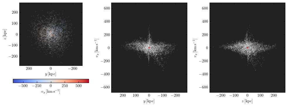
source.preview(fig=1)  # uses matplotlib `plt.figure(1)`

The preview function returns the Figure object, so this can be captured manipulated, if desired. The resulting preview looks like:

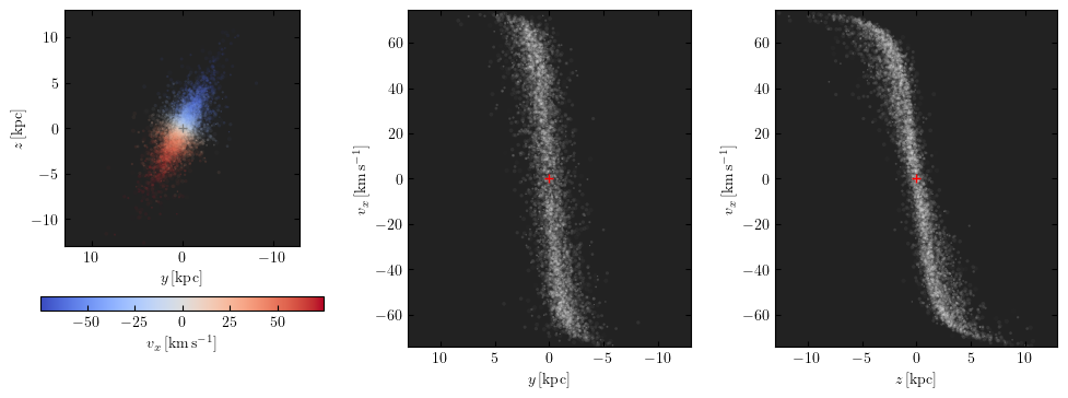
The number of particles plotted is limited to 5000 to avoid excessively large Figure objects, but this can be controlled with the max_points keyword argument. The first panel shows the particle positions in the y-z plane (which approximately maps to RA and Dec), coloured by the x-component of the velocity (which approximately maps to the line-of-sight velocity). The second panel shows the PV diagram of particle along the y coordinate direction, and the third panel the same along the z coordinate direction. Let’s rotate the disc to be edge on and preview it again:

from martini import L_coords
source.rotate(
    L_coords=L_coords(incl=90 * U.deg, az_rot=0 * U.deg, pa=270 * U.deg)
)
source.preview(fig=2)

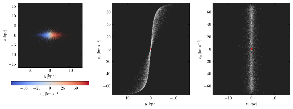
This does look like an edge on disc, and the PV diagrams now correspond to the major (middle panel) and minor (right panel) axis PV diagrams. Let’s switch orientations again to 60 degrees inclined and a position angle offset 45 degrees from its previous value of 270 degrees, and this time we’ll show only 100 points.

source.rotate(L_coords=L_coords(incl=60 * U.deg, az_rot=0 * U.deg, pa=225 * U.deg))
source.preview(max_points=100, fig=3)

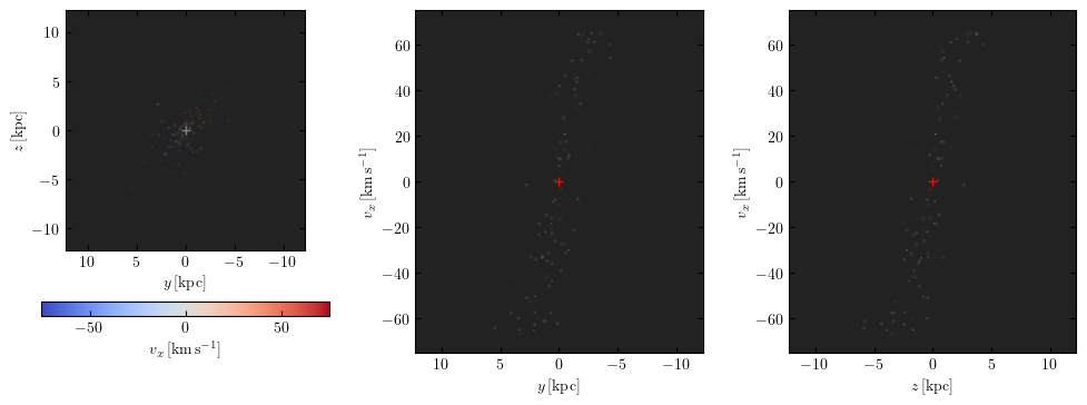
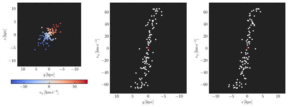
This doesn’t look great. The preview function tries to adjust the transparency and sizes of the points to qualitatively reflect their HI masses and smoothing lengths, but this may sometimes lead to results that aren’t very useful. The points can be forced to a constant size and transparency with point_scaling="fixed".

source.preview(max_points=100, fig=4, point_scaling="fixed")

Let’s look at a more realistic example from the TNG simulations.

from martini.sources import TNGSource

tng_source = TNGSource(
    "TNG50-1",
    99,
    572840,
    api_key="your-tng-api-key-goes-here",
)
tng_source.preview(fig=5)

The preview function scales the axes to enclose all particles in the source. In this case we’re mostly seeing the hot circumgalactic gas extending out beyond 200 kpc. The lim keyword argument sets the (absolute value) offset from the centre shown in the preview, and the vlim keyword argument similarly limits the velocity offset from zero. Note that these keyword arguments have no influence on the particles contained in the source, just on what’s visible in the preview. Let’s take a guess at the likely size of a disc and see what’s there.

tng_source.preview(fig=6, lim=20 * U.kpc, vlim=300 * U.km / U.s)

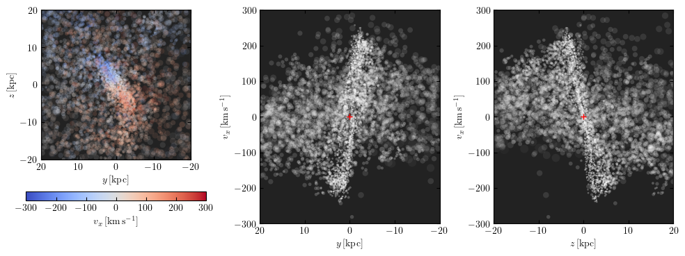
Aha, an inclined disc within the hot halo. From here we could continue to adjust the orientation, if desired.

Because the TNGSource module has automatically retrieved and loaded the particle arrays, we did not need to pass them in, and therefore never had a chance to do anything with them, if we desired to. The particle arrays are accessible as attributes, for example:

tng_source.coordinates_g  # positions and velocities
tng_source.mHI_g
tng_source.T_g
tng_source.hsm_g

The same attributes exist for all source modules available in MARTINI. The positions and velocities are stored using features of the astropy.coordinates module to help manipulate them. The positions and velocities can be accessed like this:

tng_source.coordinates_g.get_xyz()  # positions
tng_source.coordinates_g.differentials["s"].get_d_xyz()  # velocities